Enigmatic Election
4/25/2021
Problem Statement
The Riddler election problem stated here asks:
Riddler Nation’s neighbor to the west, Enigmerica, is holding an election between two candidates, A and B. Assume every person in Enigmerica votes randomly and independently, and that the number of voters is very, very large. Moreover, due to health precautions, 20 percent of the population decides to vote early by mail. On election night, the results of the 80 percent who voted on Election Day are reported out. Over the next several days, the remaining 20 percent of the votes are then tallied. What is the probability that the candidate who had fewer votes tallied on election night ultimately wins the race?
Answer: 15%.
Defining the Problem
I found this to be an exceedingly challenging issue to solve analytically and in the end gave way to a monte carlo solution. Some thoughts are documented here that may later be useful to solve this in closed form.
First, let's just write a few things we know to be true about the problem in general. On election night, 80% of the votes in some infinitely large population are tallied. All votes are random and independent, which by definition means that the expected propensity to vote for candidate A and B is 50%. This expected propensity must be true in the 80% subset and also in the 20% subset and we do not assume there is anything systematically different about the 20% subset or the 80% subset that makes them more likely to vote for either candidate differentially.
With this statement, then we know that each election is just one draw from the true distribution of possible outcomes and while in expectation each candidate has a 50% chance of winning, no given draw will be exactly 50%. So, each draw has some measurement error. We assume the winner is the candidate with greater than 50% of the votes. Because each candidate has the same probability of winning on election night, the only way in which the election night loser can overtake the provisional winner is by winning enough votes in the remaining 20% sample to cover the spread. Hence, the question then becomes does the candidate that lost on election night receive enough votes in the remaining 20% to cover the gap necessary to receive more than 50% of the total votes?
So, let's define a few things. Let \(N = N_{80} + N_{20}\) where \(N_{80}\) is the number of votes on election night and then \(N_{20}\) is the number of votes in the remaining 20% sample. We can then also assume that since each voter in expectation has a 50% on election night, then winning on that night is a function of measurement error. Let's denote that error as \(\epsilon\) such that the proportion of votes given to the winner on election night is \(W_{80} = .50 + \epsilon\) where \(W_{80}\) is used to mean the proportion of votes awarded to the provisional winner on election night and \(\epsilon\) is a very small, positive number such that as \(N \rightarrow \infty\) then \(\epsilon \rightarrow 0\), but \(\epsilon\) could never be 0 otherwise election night would be a tie. Losing that same night is the complement, so we can write \(L_{80} = 1 - W_{80}\).
Both candidates have the same expected probability of winning on election night, 50%. But, stochastically, this will not be true with one observed election. The winner will be "lucky" and receive that small stochastic bump of the votes on election night. Using these, we can then write the condition defining how many votes the election night loser must receive in the remaining 20% sample in order to win overall. That can be written as $$ V_{20} = \texttt{ceiling}\left(\left(\frac{N}{2} + 1\right) - L_{80} \times N_{80}\right) $$ where I take the ceiling to make sure it's always an integer (no fractional humans). The number \(V_{20}\) represents the number of votes needed for the candidate who lost on election night to end up winning overall. In other words, if the candidate who lost on election night receives at least \(V_{20}\) in the remaining 20% sample, that person will end up with more than 50% of the total vote share, and will become the winner. That is, $$ \frac{L_{80} \times N_{80} + V_{20}}{N} > .50 $$
Now, it is still true that in the remaining 20% sample, both candidates have a 50% chance of winning, but the losing candidate must now win at least \(V_{20}\) votes in the 20% sample, which is more than 50% of the remaining votes. This implies we need to integrate over some probability distribution function with the problem stated generically as $$ \Pr(X \geq V_{20}) = \int_{V_{20}}^{N_{20}} f(x)dx $$
which in this context would be summation over discrete numbers if assuming binomial or I can use continuous since the normal is a good approximation of the binomial in this instance. The challenge though is that with increasing \(N\), \(V_{20}\) represents only \(.5 + \epsilon\) of the votes in the remaining 20% sample. So, if that distribution is symmetric in any way, then well, you get 50% and that's not right. So, in the end I let the computer run for a very long time to find how this plays out conceptually. I set \(N=1,000,000\) and then ran 100,000 replicates of the problem. Reproducible R code below which returns 15%.
N <- 1000000
K <- 100000
overall <- numeric(K)
for(i in 1:K){
	vote80 <- rbinom(N*.8, 1, prob=.5)
	vote20 <- rbinom(N*.2, 1, prob=.5)
	### Who lost on election night
	aTable <- table(vote80)
	result1 <- names(which.min(aTable))
	### Who wins overall after 20% are added in
	theTable <- table(c(vote80,vote20))
	result2 <- names(which.max(theTable))
	overall[i] <- result1 == result2
}
### How often does this occur (this is probability)
mean(overall)
Endlessly Pouring Water
4/10/2021
Problem Statement
The Riddler water cup problem stated here asks:
You have two 16-ounce cups — cup A and cup B. Both cups initially have 8 ounces of water in them. You take half of the water in cup A and pour it into cup B. Then, you take half of the water in cup B and pour it back into cup A. You do this again. And again. And again. And then many, many, many more times — always pouring half the contents of A into B, and then half of B back into A. When you finally pause for a breather, what fraction of the total water is in cup A? Extra credit: Now suppose both cups initially have somewhere between 0 and 8 ounces of water in them. You don’t know the precise amount in each cup, but you know that both cups are not empty. Again, you pour half the water from Cup A into Cup B, and then half from Cup B back to A. You do this many, many times. When you again finally pause for a breather, what fraction of the total water is in Cup A?
Answer: The express is a special case of its extra credit, so they both have the same answer of \(\frac{2}{3}\approx 0.6666667 \). Below I show how to arrive at the following expression to find the fraction of water in Cup A at the \(n\)th trial $$ \frac{1}{2} + \frac{1}{2} \sum_{i=1}^n \left(\frac{1}{4}\right)^i $$ This expression is useful for learning what the value would be at specific values of \(n\) where \(n\) might be finite. But, we can take the limit of the portion $$ \begin{split} \lim_{n \to \infty} \left(\sum_{i=1}^n \left(\frac{1}{4}\right)^i\right) = \frac{1}{3} \end{split} $$ Giving a simple expression for the expected value in a more computationally tractable way $$ \frac{1}{2} + \frac{1}{2}\times\frac{1}{3} = \frac{2}{3} $$
Defining the Problem
In this problem we're wandering through the state space of just pouring back and forth between the two cups. Conceptually, we can start by knowing that in the first step, we take half of the water in Cup A (it originally starts with 8 ounces) and pour it into Cup B which also originally starts with 8 ounces. So, Cup B would now have 12 ounces and Cup A now has 4 ounces. OK, now we repeat and pour half of the water in Cup B back into Cup A, which now has 10 ounces. So, at this step, Cup A has \(\frac{10}{16} = .625\), or 62.5% of the water. But, that was just two pours and we need to do this many more times.
It's helpful to think step by step because then we realize the amount of water in the cup depends on the prior state of the two cups, a bit of Markovian thinking. Perhaps start with a small simulation to "see" how this plays out numerically in a few trials.
Manually Create Transition Matrix
We could write some R code to manually do this \(n\) times and observe what fraction would be in Cup A after a certain number of trials. It's burdensome, but here is what we would observe. The rows in the matrix \(X\) below are the proportions of water in each cup and each new row depends on the proportions in the row just above it. In this we just deal wth the proportions directly and no need to deal with ounces.
The initial state begins with both cups having an equal share of water and then State 1 shows Cup A would have 25% of its water remaining and Cup B would now have 75% of the water. Then, pouring half from Cup B back to into Cup A we see that in State 2 Cup A would have 62.5% of the water (.75/2 + .25 = .625) and so on until we take a break after 18 states, pour half of Cup B back into Cup A and the final step shows about 67% of the water is now in Cup A.
#### Iterate
X <- matrix(0, 19,2)
X[1,] <- c(.5, .5) # start
L <- seq(1,nrow(X)-2,2)
for(i in L){
	X[(i+1),] <- c(X[i,1]/2, X[i,2] + X[i,1]/2) # pour A into B
	X[(i+2),] <- c(X[(i+1),1] + X[(i+1),2]/2, X[(i+1),2]/2) # pour B into A
}

X <- data.frame(X[-1,])
X$Note <- gl(2, 1, 18, labels = c('Pour B into A', 'Pour A into B'))
colnames(X) <- c('Fraction in A', 'Fraction in B', 'Pour Direction')
> X
   Fraction in A Fraction in B Pour Direction
1      0.2500000     0.7500000  Pour A into B
2      0.6250000     0.3750000  Pour B into A
3      0.3125000     0.6875000  Pour A into B
4      0.6562500     0.3437500  Pour B into A
5      0.3281250     0.6718750  Pour A into B
6      0.6640625     0.3359375  Pour B into A
7      0.3320312     0.6679688  Pour A into B
8      0.6660156     0.3339844  Pour B into A
9      0.3330078     0.6669922  Pour A into B
10     0.6665039     0.3334961  Pour B into A
11     0.3332520     0.6667480  Pour A into B
12     0.6666260     0.3333740  Pour B into A
13     0.3333130     0.6666870  Pour A into B
14     0.6666565     0.3333435  Pour B into A
15     0.3333282     0.6666718  Pour A into B
16     0.6666641     0.3333359  Pour B into A
17     0.3333321     0.6666679  Pour A into B
18     0.6666660     0.3333340  Pour B into A
A More Concise Solution
Using the code above we could wander the state space and we could find the fraction of water in Cup A at any point. But, who wants to stare at matrices and find values in rows! So, instead we can find the exact fraction of water in Cup A at any point using the following solution $$ \frac{1}{2} + \frac{1}{2} \sum_{i=1}^n \left(\frac{1}{4}\right)^i $$
> 1/2 + 1/2 * sum((1/4)^(1:50))
[1] 0.6666667
Here is just a snippet of how to arrive at this conceptually. If we were to manually write out the proportion of water in Cup A at each step we would manually write the first three steps as
> a <- b <- .5
> ((1- (a)/2) + (a))/2
[1] 0.625
> (1- (((1- (a)/2) + (a))/2)/2)/2 + (((1- (a)/2) + (a))/2)/2
[1] 0.65625
> (1-(((1- (((1- (a)/2) + (a))/2)/2)/2 + (((1 - (a)/2) + (a))/2)/2)/2))/2 + ((1- (((1- (a)/2) + (a))/2)/2)/2 + (((1- (a)/2) + (a))/2)/2)/2
[1] 0.6640625
Note, these values match those in the transition matrix \(X\) for the first three instances of where Cup B is poured back into Cup A. Let's simplify and rearrange each step to yield
a <- .5
> 1/2 + a/4
[1] 0.625
> 1/2 + a/4 + a/16
[1] 0.65625
> 1/2 + a/4 + a/16 + a/64
[1] 0.6640625
We get that "aha" moment when we realize the accumulations are in the pattern
$$
\frac{1}{2} + \frac{a}{4} + \frac{a}{16} + \frac{a}{64} \ldots
$$
where \(a\) = .5. So, we can simply sum over the sequence of \(n\) steps and find exactly what fraction of water is in Cup A at any specific point. Let's clean this up and generalize.
A Final Computational Solution
Summation of the multiple exponents is useful if I want to know what the fraction would be after a specific trial. However, supposing I want to assume it's summation over an extremely large number of trials, summing over exponents is computationally expensive with increasing \(n\). So, as shown in the introduction, we can reduce to a very simple computation after taking the limit as the summation approaches a very large number $$ \frac{1}{2} + \frac{1}{2}\times\frac{1}{3} = \frac{2}{3} $$
Last, we can run a small monte carlo simulation just to see how well this all works out. In this below, Cup A starts with a random amount of water and then Cup B has a random amount such that the total amount of water sums to 1.
cupa <- runif(1)
cupb <- 1 - cupa
total <- cupa + cupb
K <- 2000
resulta <- numeric(K)

for(i in 1:K){
	## pour half of A into B
	cupb <- cupa * .5 + cupb
	## Account for removal in cupa
	cupa <- cupa * .5

	### now pour half of B into A
	cupa <- cupb *.5 + cupa
	## Account for removal in cupb
	cupb <- cupb * .5
	resulta[i] <- cupa
}
resulta[K]
Riddler Ski Federation
1/23/2021
Problem Statement
The Riddler Ski Federation problem stated here asks:
Each of you will complete two runs down the mountain, and the times of your runs will be added together. Whoever skis in the least overall time is the winner. Also, this being the Riddler Ski Federation, you have been presented detailed data on both you and your opponent. You are evenly matched, and both have the same normal probability distribution of finishing times for each run. And for both of you, your time on the first run is completely independent of your time on the second run. For the first runs, your opponent goes first. Then, it’s your turn. As you cross the finish line, your coach excitedly signals to you that you were faster than your opponent. Without knowing either exact time, what’s the probability that you will still be ahead after the second run and earn your gold medal?
Answer: 75% from simulation and about 75.3% from "exact" although exact approaches still require approximations for order statistics from normal.
Defining the Problem
Define some notation and let \(s_{ij}\) denote the time of skier \(i =\{1,2\}\) on attempt \(j =\{1,2\}\). The problem statement indicates that both skiers share the same true ability distribution \(s_{ij} \sim \mathcal{N}(\mu, \sigma^2)\). Hence, each run down the slopes represents one random draw from that ability distribution.
On attempt 1 we always observe the condition \(s_{11} < s_{21}\). That is, you did better by some measure than your opponent. However, we can assume that the time for either athlete on attempt 2 can be any random draw from \(s_{i2}\sim \mathcal{N}(\mu, \sigma^2)\) with no particular ordering. So, from the onset we know we are dealing with order statistics from the normal distribution. We will end up needing the 1st and 2nd order statistics in a sample of size 2 from the normal.
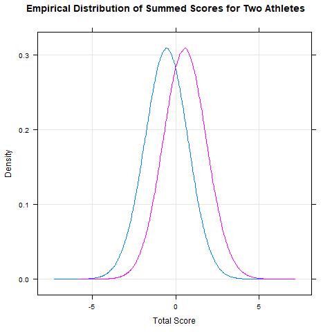
Now the winner is the athlete with the best overall time. So, we would add both times together and the lower of the two summed scores is the overall winner. Let the total summed scores be denoted as \(s^*_{1} = s_{11}+ s_{12}\) and \(s^*_{2} = s_{21}+ s_{22}\). We can now phrase our problem conceptually as we seek the probability that the total overall score for skier 1 (you) is faster than the total overall score for skier 2 given that you always placed first on the initial run. We can write the following as the probability we wish to obtain: $$ \Pr(s^*_{1} < s^*_{2}) = \Phi\left(\frac{s^*_{2} - s^*_{1}}{ \sqrt{\sigma^2_{s^*_{1}} + \sigma^2_{s^*_{2}}}}\right) $$ where \(\Phi(\cdot)\) is the normal CDF (justification for normal provided below). Estimating this probability requires having expected values for both of the summed timings, \(s^*_{i}\), and their variances. So, now we need to implement an approach to obtain those expected values.
Of course, the individual values for \(s_{ij}\) are latent. But, we can build up a way to answer the problem via their expected values and variances. We have enough information to know that the expected value for \(s_{11}\) will be the 1st order statistic from a normal with a sample of size 2 and the expected value for \(s_{21}\) will be the 2nd order statistic from a normal with a sample of size 2. Both \(s_{i2}\) will share a common expected value because they are drawn from the same ability distribution.
Without loss of generality, I assume that the parameters of the normal are \(\mu =0\) and \(\sigma^2 = 1\) in order to identify a solution in all that follows.
First A Simulation
We can simulate the nature of the problem and arrive at an answer and it then leads to a few interesting things to then consider so we can formulate a more exact solution. First, take two random draws from \(s_{i1}\sim \mathcal{N}(0,1)\) for attempt 1 and always assign the lower time to \(s_{11}\). This guarantees that both times are drawn from the same ability distribution, but implements the ordering condition that \(s_{11} < s_{21}\). The Riddler problem is about times down the slope, and so these random draws can be viewed as some scaled metric for time with the lower value representing the faster time.
Now for attempt 2, again take two random draws \(s_{i2}\sim \mathcal{N}(0,1)\) and no sorting is needed at this point and form \(s^*_{1} = s_{11}+ s_{12}\) and \(s^*_{2} = s_{21}+ s_{22}\). Repeat \(K\) times and find the number of times when \(s^*_{1} < s^*_{2}\). The R code implements this below and yields a solution of 75%.
K <- 100000
run1 = t(replicate(K, sort(rnorm(2))))
run2 = t(replicate(K, rnorm(2)))
overall <- run1 + run2
table((overall[,1] < overall[,2]))/K
   FALSE     TRUE
0.249641 0.750359
Now Something More Formal
Now, it's useful to examine the mean over all \(K\) replicates from the simulation above of the values from the first run (when things are ordered). Taking the mean over all random draws from run 1 we observe values of \(\bar{s}_{11}\) = -0.5636047 for skier 1 and \(\bar{s}_{21}\) = 0.5656139 for skier 2. These are the expected values of the 1st and 2nd order statistics in a sample of size 2 from a normal distribution obtained from a monte carlo approach.
> apply(run1,2,mean)
[1] -0.5636047  0.5656139
There are also a few direct ways to calculate those order statistics. One option is that we can get the 1st and 2nd order statistics in a sample of size 2 from a normal distribution using the method by J.P. Royston (1982). An implementation of this formula in R yields
library(EnvStats)
> evNormOrdStatsScalar(r=1,n=2, method="royston")
[1] -0.5641896
> evNormOrdStatsScalar(r=2,n=2, method="royston")
[1] 0.5641896
Immediately we observe that the Royston direct calculation is the same (within stochastic limits) of the values we obtained through our monte carlo approach. Alternatively, we could use Blom's (1958) approach for the 1st and 2nd order statistics in a sample of size 2 from the normal. This is slightly less numerically precise than Royston as shown below. However, the point in showing this is that the order statistics from a normal are approximations with different approaches and those approximations may yield slightly different expected values so arriving at an "exact" answer is limited by this approximation.
# Blom
> qnorm((c(1,2) -.375)/(2-2*.375+1))
[1] -0.5894558  0.5894558
Recall there is no ordering of the times in attempt 2. We assume random draws from \(s_{i2}\sim \mathcal{N}(0, 1)\) for both athletes on attempt 2. In this case, the expected value is fixed at 0 for both athletes, though it can be any number. We can see this is true by taking the means from run 2 in our simulation.
> apply(run2,2,mean)
[1] -0.0002495554 -0.0000544851
We now have the exact values we need to form the expected summed score. Those components are \(E(s_{11}) = -0.5641896\), \(E(s_{21}) = 0.5641896\) and \(E(s_{i2}) = 0 \ \forall \ i\). Conveniently, the total score, \(s^*_{i}\), is the sum of two components and both of those components are individually drawn from a normal distribution. This is nice because the sum of two normally distributed variables is also itself normally distributed. So, we know that our summed score term will have the property:
$$
s^*_{i} \sim \mathcal{N}(\mu_{i1} + \mu_{i2}, \sigma^2_{i1} + \sigma^2_{i2}).
$$
where \(\sigma^2_{i1}\) is the variance of the times on run 1 for athlete \(i\) and \(\sigma^2_{i2}\) is the variance on run 2 and \(\mu_{i1}\) and \(\mu_{i2}\) are the expected values, \(E(s_{i1})\) and \(E(s_{i2})\), respectively. Formally, \(\sigma^2_{i1}\) is the variance of the \(k\)th order statistic.
Pulling all of these things together, we can insert our expected values into the probability expression and use the normal CDF as:
$$
\Pr(s^*_{1} < s^*_{2}) = \Phi\left(\frac{s^*_{2} - s^*_{1}}{ \sqrt{\sigma^2_{s^*_{1}} + \sigma^2_{s^*_{2}}}}\right)
$$
Using the expression for the variance of the \(k\)th order statistic here yields an exact answer of 75.3%.
Last is a nice visual of the empirical distributions of the summed scores over \(K\) replicates.
pnorm((0.5641896 - (-0.5641896))/ sqrt(1.3583016 + 1.3583016))
[1] 0.7532043
Here is the extra credit code:
K <- 100000
run1 = t(replicate(K, sort(rnorm(30))))
run2 = t(replicate(K, rnorm(30)))
overall <- run1 + run2
table(sapply(1:nrow(overall), function(i) which.min(overall[i,])))[1]/K
   1
0.31411
The Flute-iful Challenge
1/16/2021
Problem Statement
The flute-iful challenge problem stated here asks:
You’re a contestant on the hit new game show, “You Bet Your Fife.” On the show, a random real number (i.e., decimals are allowed) is chosen between 0 and 100. Your job is to guess a value that is less than this randomly chosen number. Your reward for winning is a novelty fife that is valued precisely at your guess. For example, if the number is 75 and you guess 5, you’d win a $5 fife, but if you’d guessed 60, you’d win a $60 fife. Meanwhile, a guess of 80 would win you nothing. What number should you guess to maximize the average value of your fifing winnings?
Answer: $50.00
A Solution
Let's play this conceptually in a simple way as if there were multiple contestants to see who would have the best outcome. Begin with \(\mathbb{R}_{0 < x < 100} = \{x \in \mathbb{R}| 0 < x < 100\}\) which is used to mean the value of the random draw, \(x\), is any real between 0 and 100 and let \(g_i\) be used to denote a guess by contestant \(i\).
Suppose there are \(i = \{1, 2, \ldots, N\}\) total contestants and each contestant has a unique guess. Then, the winners are all of those in the set where \(A = \{g_i < x\}\) but the winner with the best outcome is the contestant with the maximum value of \(g_i\) in the set \(A\), or the largest guess in the set of values less than \(x\). So conceptually, we can think of everyone in the set \(A\) as a winner, but we want to find the best (richest) winner and if we knew the value of \(x\) the winner with the best outcome is the individual \(i\) who guessed just under the value of the random draw.
One way to approach the problem is to directly compute the expected value of the return for each possible value between 0 and 100. The uniform has a simple cumulative distribution function (CDF), so we know that if we were to guess $1.00, we would win 99% of the time, if we were to guess $5.00 we would win 95% of the time and so on. If the game were repeated say 1,000 times, then a $1.00 guess would only give a return of $990, but a $5.00 guess would give an expected return of $4,750! So, even though the expected occurence of winning with a $5.00 wager is less than a $1.00 wager, the average expected return on the $5.00 guess is bigger.
We can sort of brute force our way through each calculation as \(p(x) \times x\) where \(x\) is the value of the wager with corresponding probability \(p(x)\). The visual display shows where our expected return peaks. We observe that as we approach $50.00, our expected return goes up and as we go above $50.00 our expected return goes back down.
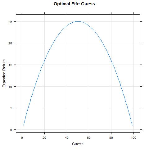
More formally I suppose we could define our function: $$ f(x) = x \left[1 - \frac{x}{100}\right] $$ and then differentiate the function: $$ f(x)' = 1 - \frac{x}{50} $$ To find its peak (i.e., where the slope is 0) set to 0 and solve yields a peak at 50.
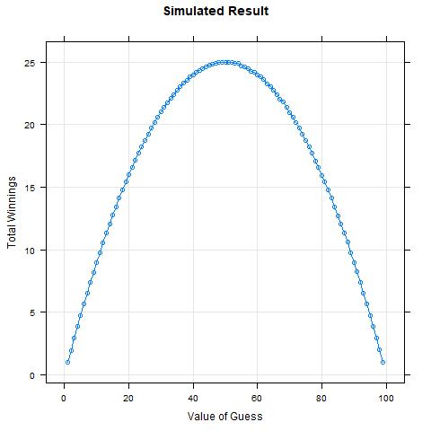
So, now let's simulate and verify this thinking is accurate.
fife <- function(guess, k = 1000000){
	value <- runif(k,0,100)
	win <- guess < value
	mean(win) * guess
}
result <- sapply(1:99, function(i) fife(i))
The Price is Right
10/18/2020
Problem Statement
The Price is Right (TPIR) problem stated here asks:
Assume the true price of this item is a randomly selected value between 0 and 100. (Note: The value is a real number and does not have to be an integer.) Among the three contestants, the winner is whoever guesses the closest price without going over. For example, if the true price is 29 and I guess 30, while another contestant guesses 20, then they would be the winner even though my guess was technically closer. In the event all three guesses exceed the actual price, the contestant who made the lowest (and therefore closest) guess is declared the winner. I mean, someone has to win, right? If you are the first to guess, and all contestants play optimally (taking full advantage of the guesses of those who went before them), what are your chances of winning?The answer is effectively 0% for player 1 if both player 2 and 3 use the cut-off strategy and they are mean. Below I show that the actual probability depends on the value for \(\epsilon\) and assumes players 2 and 3 collude to maximize thier potential gain. Specifically, the probability for player 1 to win is: $$ P(g_1) = \frac{[(g_1 + \epsilon) - (g_1 - \epsilon)]}{100} $$
The idea below is that players 2 and 3 collude to force a boundary around the guess of player 1 making it such that player 1 can only be right if they choose the exact right answer, otherwise players 2 and 3 share the remaining win chances by eliminating player 1. Hence, as \(\epsilon\) becomes smaller (but never 0), this forms a tight boundary such that the likelihood of a win for player 1 tends to 0.
Some Exploratory Ideas and Existing Research in TPIR
There is some previously existing research on this topic borrowing from game theory. Ben Blatt describes his approach for optimal Contestant Row here and provides a cheat sheet for many TPIR games here.
The generalized optimal strategy, he writes, is for the last player to bid one dollar higher than the highest of any other bid made. This increases the chances that the last player will win to 53.8%. Let's refer to this as the "last player approach", or LPA.
Scott Rick describes a "cut-off" strategy here, which strategizes in a way that precludes another player from winning at all.
In the current context, we don't have any information about the retail value of the item. Also, the rules are slightly different than the real world game in that if all bidders are over, the closest bidder is the winner. So player 1 can form any guess between 0 and 100 with equal probability. Let's use \(\mathbb{R}_{0 < p < 100} = \{p \in \mathbb{R}| 0 < p < 100\}\) to mean the price is any positive real number between 0 and 100 and then \(\mathbb{R}_{0 < g_i < 100} = \{g_i \in \mathbb{R}| 0 < g_i < 100\}\) to mean that the guess for contestant \(i = \{1,2,3\}\) is also a real in the same domain as the price.
The twitter back and forth on this game clarifies that guesses can be any real number and that player 2 can predict what player 3 will do and factor that into their gaming.
Since we are considering some general properties of this game we know the first player could only choose randomly in the absence of any information, but the other players will not use random guesses if they use an optimal strategy. So, in frequentist expectation, we can take the first guess to be: $$ E(g_1) = .5 \times (a+b) = .5 \times (0+100) = 50 $$ if player 1 in fact guesses randomly. If we apply the LPA as suggested by Blatt then player 2 will guess 51. However, since the last bidder intends to maximize their approach, they would combine both the cutoff strategy and also the LPA to make a final bid. Let \(\epsilon\) be some infinitesimally small value such that \(51 + \epsilon > 51\).
In this way, player 3 has effectively prevented player 2 from ever winning the game unless that player chooses the exact right price. This essentially makes it a game only between two players, player 1 and player 3.
Let's explore what happens if this strategy is applied using simulation. R Code below (the function tpir is provided below) implements this approach and sets \(\epsilon = .00001\). In this code, player 1 guesses 50, player 2 guesses 51, and then player 3 guesses 51 + \(\epsilon\). The result yields a 51% chance for player 1 and a 49% chance for player 3 and player 2 has been elimated, as expected.
e <-.00001
tpir(50,51,51+e, K=1000000)
winner
     1      3
50.965 49.035
Let's assume now that in contrast, player 2 knows that player 3 will use a very deterministic way of playing and always use the LPA. A smart player 2 would then drive the second price up to 99.99 such that player 3 must always bet 100. This now yields a benefit for player 2 and eliminates player 3, but highly favors player 1. This strategy would yield a 99.99% win probability for player 1 and a .01% win probability for player 2. Player 3 would be entirely eliminated as expected.
tpir(50,99.99,100, K=1000000)
winner
      1       2
99.9909  0.0091
Of course, Player 3 won't be bullied!! So, if player 2 makes this move, then player 3 would bid the other extreme, $1.00. Simulation code below shows how this scenario plays out. In this case, player 1 has a 50% chance, player 3 has a 49.95% chance and then player 2 has about a .009% chance.
tpir(50,99.99,1, K=1000000)
winner
      1       2       3
50.0342  0.0087 49.9571
Of course, player 2 knows that if they bid such a ridiculously high bid player 3 would respond similarly. Perhaps instead, the second player uses the LPA and then player 3 dives under player 1 by 1 dollar, thus ignoring the advice of Blatt. In this scenario, we would observe a 49% chance of winning by player 2 a 50% chance for player 3 and then only a 1% chance of winning by player 1.
tpir(50,51,49, K=1000000)
winner
      1       2       3
 0.9986 48.9946 50.0068
So far player 1 has been treated rather unfairly and bullied around. In fact, player 1 knows something about expected values and properties of uniform distributions. So, player 1 surmises that the expected value of the price will be $50.00 and strategically chooses \(50 - \epsilon\). The other players follow the LPA sequentially. This would yield a 50% chance for player 1, a 1% chance for player 2 and a 49% chance for player 3.
e <-.00001
tpir(50-e,50+e,51+e, K=1000000)
winner
      1       2       3
49.9514  1.0120 49.0366
However, in the end, the players want to maximize their own profit--they are not interested in sharing the gain. So, both players 2 and 3 can completely eliminate player 1 by choosing values directly under or above player 1 and split the win probability between the two of the (almost) entirely. It no longer matters what player 1 guesses, players 2 and 3 can eliminate player 1.
So, let's assume player 1 chooses $50. Then, player 2 in turn dives just under this number, \(50 - \epsilon\) and player 3 goes just above, \(50 + \epsilon\). In other words, their strategy is to form boundaries around player 1 such that the only chance of winning is if player 1 chooses the exact right number. Formally, the probability that player 1 chooses the exact right number when the other players use the cut-off strategy is: $$ P(g_1) = \frac{[(g_1 + \epsilon) - (g_1 - \epsilon)]}{100} $$
Again, simulating to observe an outcome if this strategy was used eliminates player 1 as expected and yields the largest possible gain for players 2 and 3:
e=.000001
tpir(50,50-e,50+e, K=1000000)
winner
      2       3
49.9095 50.0905
Generally, players 2 and 3 know that they can always eliminate player 1. But, if player 1 chooses a low value, say $1, then player 2 would live with \(1-\epsilon\) because if they choose \(1+\epsilon\) then player 3 would choose \(1+2\times\epsilon\), thus eliminating player 2.
### R Code function
tpir <- function(player1,player2, player3, K){
	winner <- numeric(K)
	for(i in 1:K){
		price <- runif(1,0,100)
		guesses <- c(player1, player2 , player3)
		### Who is lower and closest
		if(any(guesses < price)){
			less <- which(guesses < price)
			winner[i] <- which(guesses==guesses[less][which.min(price-guesses[less])])
		} else {
			winner[i] <- which.min(guesses - price)
		}
	}
	table(winner)/K * 100
}
Parallel Parking
10/09/2020
Problem Statement
The parallel parking problem stated here asks:
Every weekend, I drive into town for contactless curbside pickup at a local restaurant. Across the street from the restaurant are six parking spots, lined up in a row. While I can parallel park, it’s definitely not my preference. No parallel parking is required when the rearmost of the six spots is available or when there are two consecutive open spots. If there is a random arrangement of cars currently occupying four of the six spots, what’s the probability that I will have to parallel park?The answer is 40%.
Motivating Example
Consider that we have ordered parking spots 1, 2, 3, 4, 5, and 6. Let 1 represent the first parking spot and let 6 represent the rearmost spot. The driver does not need to parallel park when two adjacent spots are available or when the rearmost spot is available. So, the number of arrangements where parallel parking is not needed in this small example is countable. This would include:
2 and 3
3 and 4
4 and 5
5 and 6
6 and 1 or 2 or 3 or 4
We can see there will always be \(n-1\) adjacent spots when there are \(n\) total spaces plus the rearmost at the end with any of the other non-adjacent spots. So that means there are \(p = 5 + 4 = 9\) ways to not parallel park (i.e., 5 consecutive and 4 ways the rearmost spot would also be open with another non-adjacent). Now we need to consider the total number of ways in which the available spots can be arranged.
Towards a Solution
At this point, we need to only know the total number of possible arrangements, let this be denoted as \(M\). Since the cars park randomly into 4 of the 6 spots, the total number of possible parking arrangements is simply \(M = {n \choose k}\) where \(n\) is the total number of spaces and \(k\) is the number of spaces randomly taken. Then there are \(L = M - p\) conditions when you must parallel park.
So, the total number of possible arrangements is: $$ M = {n \choose k} = {6 \choose 4} = 15 $$
Then we have \(L = 6\) and \(M=15\), giving $$ \Pr(x) = \frac{L}{M} = \frac{6}{15} = .4 $$Some R code to simulate
spots <- 1:6
k <- 100000
count <- numeric(k)
for (i in 1:k){
	taken <- sort(sample(spots,4))
	empty <- which(!spots %in% taken)
	count[i] <- ifelse(6 %in% empty | diff(empty) == 1, 0, 1)
}
mean(count)
[1] 0.40268
Eating All The Chocolates
10/03/2020
Problem Statement
The eating chocolate problem stated here asks:
I have 10 chocolates in a bag: Two are milk chocolate, while the other eight are dark chocolate. One at a time, I randomly pull chocolates from the bag and eat them — that is, until I pick a chocolate of the other kind. When I get to the other type of chocolate, I put it back in the bag and start drawing again with the remaining chocolates. I keep going until I have eaten all 10 chocolates. For example, if I first pull out a dark chocolate, I will eat it. (I’ll always eat the first chocolate I pull out.) If I pull out a second dark chocolate, I will eat that as well. If the third one is milk chocolate, I will not eat it (yet), and instead place it back in the bag. Then I will start again, eating the first chocolate I pull out. What are the chances that the last chocolate I eat is milk chocolate?The answer is 50%.
The game is based on the concept of a Markov Chain where the probability of eating the next chocolate depends only on the prior chocolate eaten. Hats off to those who worked the probabilities by laying out all of the possible state transitions.
It's simple to know the probability of eating the first chocolate--that's always 80% for dark chocolate and 20% for milk chocolate. Then, our bag of chocolates is reduced to nine. At this point, we need to consider the likelihood that we miss the mark and draw a milk chocolate (2/9) which creates a little chaos. We would put that back into the bag and walk through the new state space again eating the new first draw and then successfully drawing the same as our first (new) draw and continuing or unsuccessfully doing so and having to start over yet again.
This solution walks through the state space using a simulation. Below is R code that counts the proportion of times that milk chocolate (type 2) is drawn last.
K <- 1000000
final <- numeric(K)
for(j in 1:K){
	### Original bag
	bag <- c(1,1,1,1,1,1,1,1,2,2)
	draw <- numeric(10)
	### Take first chocolate from bag
	draw[1] <- sample(bag,1)
	### "eat" the chocolate and remove from bag
	bag <- bag[-which(bag == draw[1])[1]]
	i <- 1
	### Now take next draw
	while(length(bag) > 1){
		i <- i + 1
		x <- sample(bag,1)
		if(x == draw[(i-1)]){ ### If same chocolate eat and remove
			draw[i] <- x
			bag <- bag[-which(bag == draw[i])[1]] # eat it
		} else { ### If not, put it back and start over
			x <- sample(bag,1)
			bag <- bag[-which(bag == x)[1]] # eat it
			draw[i] <- x
		}
	}
final[j] <- bag
}
table(final)/K
final
       1        2
0.499596 0.500404
Shooting Par
09/26/2020
Errata (9/28/2020). The solution below fails to convert either \(L_0\) to inches or \(L_4\) to yards. So, either set \(L_0\) = 14,400 or set \(L_4\) = 0.059027778. Then, the proposed solution stands.
Problem Statement
The shooting par golf problem stated here asks:
A typical hole is about 400 yards long, while the cup measures a mere 4.25 inches in diameter. Suppose that, with every swing, you hit the ball X percent closer to the center of the hole. For example, if X were 75 percent, then with every swing the ball would be four times closer to the hole than it was previously. For a 400-yard hole, assuming there are no hazards (water, sand or otherwise) in the way, what is the minimum value of X so that you’ll shoot par, meaning you’ll hit the ball into the cup in exactly four strokes?The answer is \(73.00243\%\) with solution below and a little interactive visual display showing where the ball would land at the fourth hit under different percentages.
Motivating Example
Conceptually, we need to set something up along the lines of the following. At the tee, I'm 400 yards away, or at the initial location, \(L_0\) = 400. From initial position, \(L_0\), I take my first swing and move the ball to the new location, \(L_1\), moving \(p\%\) closer to the destination. Now from \(L_1\) I take a second hit and land at position \(L_2\) by again moving the ball by the same percent. Repeat by hitting \(p\%\) closer to the hole each time until hit four puts me right at the edge of the hole on my side of the tee.
Since the diameter of the hole is 4.25, we can assume the ball falls into the cup once it reaches the outer edge of the cup, or is 2.125 inches from the center of the hole. Technically, we might assume the location of the final hit is represented as an inequality, \(\leq 2.125\). But, for convenience, I'll assume landing at exactly 2.125 results in a gravitional pull towards the center of the cup.
Let \(L_i\) be the location of the ball after hit \(i = \{1,2,3,4\}\) then we need to move the ball from \(L_0\) to \(L_4\) in exactly four swings and each hit moves the ball \(p\%\) closer such that: $$ p = 1- \frac{L_i}{L_{i-1}}, \ \forall \ i $$
where \(p\% = 100 \times p\).Towards a Solution
I set this up to find the best value for \(x\), then \(p = 1-x\). Start by writing the four hits as the following system of equations: $$ \begin{split} L_0 \times x &= L_1\\ L_1 \times x &= L_2\\ L_2 \times x &= L_3\\ L_3 \times x &= L_4\\ \end{split} $$
We know that \(L_0\) = 400 and \(L_4\) = 2.125, then use the method of substitution to solve for the single unknown, \(x\), in the system above resulting in: $$ \begin{split} 400 \times x^4 &= 2.125\\ x^4 &= \frac{2.125}{400}\\ x &= \left(\frac{2.125}{400}\right)^{1/4}\\ x &= 0.2699757 \end{split} $$ So hitting \(73.00243\%\) (i.e., \((1-0.2699757)\times100\)) closer to the hole each time puts me within the expected radius of the hole.
Let's plug in the value and see what would happen at each hit. Start at 400 yards away and then hitting \(73.00243\%\) closer to the hole puts me at location \(L_1 = 107.9903\). From this new point, I hit \(73.00243\%\) closer again and end up at location \(L_2 = 29.15476\). From location \(L_2\) I again shorten the distance to the hole by \(73.00243\%\) and end up at location \(L_3 = 7.871077\). Finally, with my fourth and final hit I again shorten the distance between \(L_3\) and the hole by \(73.00243\%\) and end up at \(L_4\)=2.124999.
A Visualization
The Python code helps with a brute force sense of the best value for \(p\) by examining the interactive visual and finding where the value for \(p\) approximately first intersects with the edge of the cup, or at about 2.125 at location \(L_4\). Plotly is great because you can interact with the visual and zoom into regions closer to "find" the best value (or see this visual in its own tab.
To see where the ball would land on the fourth hit for different percentages, hover over the blue line until it intersects with the green line (which represents the edge of the cup at point 2.125) and we see they seemingly first intersect right around \(73\%\).
import plotly.express as px
import numpy as np
p = np.arange(0,1,.0001)
result = 400*p**4
fig =px.scatter(x=1-p, y=result)
fig.update_layout(title='Brute Force Search Over Various Values of P%',
	xaxis_title='Value for P',
	yaxis_title='Ball Location at L_4')
fig.add_shape(
	# Line Horizontal
		type="line",
		x0=0,
		y0=2.125,
		x1=1,
		y1=2.125,
		line=dict(
			color="Green",
			width=4,
		),
)
fig.update_shapes(dict(xref='x', yref='y'))
fig.show()
Dictionary Problem
Problem Statement
The dictionary problem as stated here is summarized as: "Each secret word is randomly chosen from a dictionary with exactly 267,751 entries. If you have this dictionary memorized, and play the game as efficiently as possible, how many guesses should you expect to make to guess the secret word?" The answer is 17.04 with a maximum number of required guesses being 19.
Motivating Example
The solution is motivated by a simple example using a binary search algorithm to consider how we might work efficiently. To illustrate, I pick a random number from 1 to 15 and ask you to guess the number I am thinking. I will tell you if it's higher, lower, or correct. You first guess the midpoint, 8, which has a \(\frac{1}{15}\) chance of being correct. If the number is higher you can eliminate numbers 1 to 8 (or vice versa if the number is lower) and guess two has a \(\frac{1}{7}\) chance of being correct by focusing on the new region of the sequence (i.e., numbers 9 through 15). If a guess 3 is needed, find the midpoint in the remaining sequence and the success probability becomes \(\frac{1}{3}\). Last, guess 4 (if needed) has only one remaining possible choice, hence the success probability at this point is 1. Using this strategy with a sequence of size 15, you would need a maximum of 4 attempts to identify the number with certainty.
So, by iteratively halving the sequence and reducing the search space in the region where the number exists, we continue to improve the probability of success until we ultimately reach a point of certainty. This illustrates a way to work efficiently and a model for estimating the maximum number of guesses we would need to find a solution. However, we won't always need the maximum number of guesses as other values less than the maximum have non-zero probabilities, but this helps conceptualize the problem to work towards a solution for the expected value.
Combining these pieces of information, we can find the expected value for the number of guesses, \(E(G)\), by using the probabilities of being right or wrong at each possible guess, 1 through the maximum. In this example, we can write: $$ E(G) = 1 \cdot \frac{1}{15} + 2 \cdot \frac{14}{15}\frac{1}{7} + 3 \cdot \frac{14}{15}\frac{6}{7}\frac{1}{3} + 4 \cdot \frac{14}{15}\frac{6}{7}\frac{2}{3}1 = 3.266 $$ This example shows that piecing this together requires knowing:
- The maximum number of guesses needed
- The probability of being right at each guess
- The accumulated probabilities of being wrong for all guesses prior to the \(n\)th guess
Towards a Solution
Knowing that our success probability tends to 1 using this strategy, finding a general solution requires building a model that makes use of this efficient strategy. For completeness, first find the maximum number of times a sequence of size \(k\) can be halved: $$ L = \textrm{floor}\left(\frac{\log(k)}{\log(2)}\right) $$ and then generally the maximum number of guesses needed to locate the correct answer in a sequence of size \(k\) is \(N = 1 + L\), or initial guess plus remaining number of times the sequence can be halved. Then, generalizing to find the expected value over an arbitrary sequence of length \(k\): $$ E(G) = \Pr(x=1|g_1) + \sum_{n=2}^N \left(n \cdot \Pr(x=1|g_n) \prod_{j \in a}\Pr(x=0|g_j)\right) $$ where the notation \(j \in a\) is used to mean the accumulated set of incorrect probabilities preceding the \(n\)th guess which can be computed by recursion.
Applying this to the dictionary problem with a dictionary consisting of 267,751 words yields an expected maximum number of guesses: $$ \textrm{floor}\left(\frac{\log(267751)}{\log(2)}\right) + 1 = 19. $$
However, guessing the secret word could happen in fewer than 19 guesses. We can apply the expression above to find \(E(G) = 17.04\). Additionally, we can simulate the problem using a binary search algorithm over multiple replications of the problem and find the expected value of 17.04 via simulation. The result would give an empirical distribution for the number of guesses needed to find the secret word as:
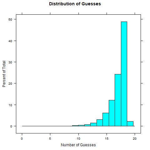
Below is R code implementing the binary search and repeating that process to find the expected value for the number of guesses.
### Function to implement binary search
### k = secret number
### s = ordered sequence
### Function searches for secret number
### and reports number of iterations to find
binSearch <- function(k, s){
	s <- 1:s
	counter <- 1
		while(length(s) > 1){
			mid <- floor(median(s))
			if (k == mid){
			s <- k
			} else if (k < mid){
			s <- min(s):(mid-1)
			counter <- counter + 1
			} else {
			s <- (mid+1):max(s)
			counter <- counter + 1
		}
	}
	list("Value Found" = s, "Number of Iterations" = counter)
}

### Iterate over binSearch function 200,000 times to find expected value
k <- 200000
result <- numeric(k)
L <- 267751
for(i in 1:k){
	x <- sample(1:L,1)
	result[i] <- as.numeric(binSearch(x,L)[2][1])
}
mean(result)
Basketball Problem
Problem Statement
The basketball problem as stated here is summarized as, "What is the probability that, on any given week, it’s possible to form two equal teams with everyone playing, where two towns are pitted against the third?"
The general answer is \(\left(\frac{1}{N}\right)^3 \left[\frac{(N-1)^2 + (N-1)}{2}\right] \times 3\) where \(N\) is the number of individuals that show up from each of the three towns randomly. Then, the case with 5 players is a special case of this such that \(\left(\frac{1}{5}\right)^3 \left[\frac{(5-1)^2 + (5-1)}{2}\right] \times 3 = .24\).
Motivating Example
It's easy to see the concept when N = 5 because the number of equal team combinations is small. In this example, we observe 30 possible ways in which equal teams could be created. For example, if 2 members show up from town \(x_1\), then we must have 1 from town \(x_2\) and 1 from town \(x_3\) (there is no option where 0 members show up from any town). So, write this as 2;1-1 as notation to mean that 2 members arrive from town \(x_1\) and then the equal team is created when 1 member arrives from town \(x_2\) and 1 more from town \(x_3\). Then, the other possible patterns in this example are 3;1-2, 3;2-1, 4;1-3, 4;2-2, 4;3-1, 5;1-4, 5;2-3, 5;3-2, and 5;4-1.
Towards a Solution
The motivating example shows a total of \(\frac{(N-1)^2 + (N-1)}{2}\) unique combinations for equal teams where town \(x_1\) is pitted against towns \(x_2\) and \(x_3\). But, since this can be arranged such that any town is the third town, we actually have \(\frac{(N-1)^2 + (N-1)}{2} \times 3\) possible equal team combinations. Since we also assume each outcome is equally as likely (i.e., any number from 1 to 5 might show up), we have a probability of \(p = \left(\frac{1}{N}\right)^3\) to observe this outcome for each of the possible combinations to make equal teams. So in words, it's the probability of the outcome times the number of times an "equal teams" outcome can occur with \(N\) players from 3 towns.
We can "check" the analytic expression with a simulation. Some R code to run a simulation over \(K\) replications of the problem where \(N\) is the upper limit on the number of players that might arrive from any given town.
### MC Answer

K <- 1000000

N <- 5 # Change this to be any number of max players

team1 <- sample(N,K, replace = TRUE)

team2 <- sample(N,K, replace = TRUE)

team3 <- sample(N,K, replace = TRUE)

full <- as.data.frame(cbind(team1, team2, team3))

indx <- apply(full, 1, function(x) which.max(x))

result <- sapply(1:K, function(i) sum(full[i, -indx[i]]) == full[i,indx[i]])

table(result)[2]/K

### Analytic

(1/N)^3 * ((N-1)^2 + (N-1))/2 * 3
The Broken Ruler Problem
Problem Statement
The broken ruler problem as stated here asks, "Recently, there was an issue with the production of foot-long rulers. It seems that each ruler was accidentally sliced at three random points along the ruler, resulting in four pieces. Looking on the bright side, that means there are now four times as many rulers — they just happen to have different lengths. On average, how long are the pieces that contain the 6-inch mark?"
The answer is 5.625. This submission provides an analytic solution and additionally a simulation-based approach.
Motivating Example
We can conceptualize the problem easily. Think about splitting the 12 inch ruler into two equal regions--a lower region below the 6 inch mark and an upper region above the 6 inch mark. Let \(R_1\) be the lower region, \(0 \leq R_1 < 6\) and let \(R_2\) be the upper region, \(6 < R_2 \leq 12\). Let each cut, \(x_i\) for \(i = {1,2,3}\), be an ordered random variable as \(0 < x_1 < x_2 < x_3 < 12\) and further assume the cuts are independent and uniformly distributed. Then there is a 50% chance that any given cut will fall into either \(R_1\) or \(R_2\).
There are only two ways in which a cut can occur containing the 6 inch mark. One potential outcome occurs when \(x_i\) \(\forall \ i\) fall into one and only one region. Then, the length is measured from the ruler's edge to the first ordered point. Refer to this as the "long cut" because we know it must be at least 6 inches in length.
A second way is when two cuts fall into one region and the remaining cut falls into the other. Then, the length is measured using the points where the 6 inch mark is interior to the cuts. For example, case 1 might be all points fall into \(R_1\) in which case the length is measured as \(L = 12 - x_3\). Or to illustrate case 2 we might observe two points in \(R_1\) and one point in \(R_2\). Then, the length is measured as \(L = x_3 - x_2\). Refer to this as the "short cut" because this slice can be less than 6 inches.
All cuts are latent random variables and so we cannot know values for \(x_i\)--the preceding is just conceptual and motivates towards a solution.
Towards a Solution
Order statistics have some nicely defined (and simple) expected values that work well for this scenario that are useful for solving this problem. It is specifically useful to know that \(E(\min(x_1, \dots, x_n ))= \frac{1}{n + 1}\). Then, we can define the expected value for the "long cut" to be: $$ 6 \times (1 + E(\min(x_1,x_2,x_3)) = 6 \times (1 + 1/4) = 7.5. $$ The probability that all three cuts fall above the 6" mark is \(.5^3\) = .125. Conversely, all cuts can fall below with the same probability, so long cuts will occur \(25\%\) of the time. Note, in this expectation I assume all values for \(x_i\) fall into region \(R_2\). But, the opposite (and similar) expected value can be written for when all values for \(x_i\) fall into region \(R_1\).
We can similarly define a "short cut" as: $$ 6 \times (E(\min(x_3,x_2) - E(x_1)) = 6 \times ((1 + 1/3) - 1/2) = 5. $$ The probability of this occuring is 1 - .25 = .75 (i.e., the converse of the long cut). Note that in this expectation, I assume both \(x_2\) and \(x_3\) fall into region \(R_2\) and then \(x_1\) falls into \(R_1\). The similar and opposite can also occur.
We've now defined the universe of potential outcomes and their probability of occuring, so to find the exact answer we then simply find the expected value via the weighted mean of the two potential outcomes: $$ \begin{split} E(X) & = \sum_{i=1}^2p_iX_i \\ & = .25 \times 7.5 + .75 \times 5 \\ & = 5.625. \end{split} $$ where \(X_i\) denotes the long and short cuts, respectively.
To "verify" lets explore using a simulation-based method. Take 3 random draws for \(x_i \sim U[0,12]\) and sort them by increasing value to represent the ordering of \(x_1, x_2\), and \(x_3\). These can be treated as the cut locations on the ruler occuring at three randomly placed locations between 0 and 12 giving us a simulated "broken ruler" with 4 segments.
Now, search to find which of the four resulting segments contains the 6 inch mark and measure the length of this segment as \(L = x_i - x_{i-1}\). Replicate this process \(K\) times, yielding a vector of lengths, \(L = {L_1, L_2, \ldots, L_k}\) and find the mean over the vector of simulated possible outcomes.
The R code below implements this process for generating the data and finding the mean. If we examine the empirical distribution of all simulated outcomes, we see a "shark fin" looking distribution of potential outcomes.
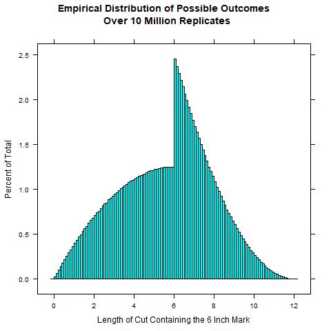
K = 10000000 #Number of replicates. Change to a lower number for speed
result <- numeric(K)
for(i in 1:K){
	### Randomly cut a ruler into 4 pieces (three random cuts)
	cuts <- c(0, sort(runif(3, 0, 12)), 12)

	### Find which piece contains 6" mark
	pos <- min(which(TRUE == (6 <= cuts)))

	### Measure length of piece containing the 6" mark
	result[i] <- cuts[pos]-cuts[(pos-1)]
}

mean(result)
5.62484
The Short Season Baseball Problem
Problem Statement
The short season baseball problem as stated here asks:
"Some statistics are more achievable than others in a shortened season. Suppose your true batting average is .350, meaning you have a 35 percent chance of getting a hit with every at-bat. If you have four at-bats per game, what are your chances of batting at least .400 over the course of the 60-game season? And how does this compare to your chances of batting at least .400 over the course of a 162-game season? Extra credit: Some statistics are less achievable in a shortened season. What are your chances of getting a hit in at least 56 consecutive games, tying or breaking Joe DiMaggio’s record, in a 60-game season? And how does this compare to your chances in a 162-game season? (Again, suppose your true batting average is .350 and you have four at-bats per game.)"
The answer is 0.0541855.
Towards a Solution
Begin with assuming each hit is an independent event so this means that the expected number of hits over 240 at bats (60 games \(\times\) 4 at bats per game) is .35 \(\times\) 240 = 84. Hitting a .400 in 240 at bats means we would observe 96 hits.
The binomial distribution gives the probability for observing independent events, but the beta distribution is the probability distribution for modeling proportions (i.e., continuous and bounded between 0 and 1). The Riddler Nation question is asking what is the probability of observing a specific proportion (e.g., chances of batting .400). So, we can easily find the shape parameters for the beta since we know the expected proportion over 240 events is .350, so then solving for \(\alpha\) and \(\beta\): $$ .35 = \frac{\alpha}{\alpha + \beta} $$ So then rearranging to solve for \(\alpha\): $$ \begin{split} \alpha & = .35\times(\alpha + \beta)\\ & = .35\times240\\ &= 84 \end{split} $$ and then \(\beta\) = 240 - 84 = 156. Now, we have a continuous p.d.f. and we can find the answer by evaluating the integral over \(f(x|\alpha, \beta) \sim Beta(84,156)\) or: $$ \begin{split} E(H) & = \int^1_{.4}f(x|\alpha, \beta)dx\\ & = 0.0541855 \end{split} $$ So, the chances are roughly about 5.4% that we would observe a batter with a true batting average of .35 hitting a .400 average in a 60 game season. Some R code to show math result:
f <- function(x) dbeta(x, 84, 156)
integrate(f, .4,1)
0.0541855 with absolute error < 6.7e-06
1-pbeta(.4, 84, 156)
[1] 0.0541855
Now using the same approach, we can answer how this compares to a true .350 batter hitting a .400 in a 162 game season. Here the shape parameters \(\alpha\) = 226.8 and \(\beta\) = 421.2 (find these using 648 total at bats in 162 games with a true .350 probability). In this case the probability that we observe a .400 season is 0.004319934, or we expect roughly a .43% chance of observing a true .350 hitter batting a .400 in a 162 game season. Some more R code:
f <- function(x) dbeta(x, 226.8, 421.2)
integrate(f, .4,1)
0.004319934 with absolute error < 4.6e-09
Out of curiosity, we might be tempted to assume that we can use a gaussian normal rather than a beta. From the properties of the binomial, we have an expected mean of 84 and a standard error of \(\sigma = \sqrt{.35\times(1-.35) \times 240)}\) = 7.389181. We could evaluate the integral over the normal from 96 to infinity, $$ \begin{split} E(H) & \approx \int^{\infty}_{96}f(x|\mu, \sigma)dx\\ & \approx 0.05218834 \end{split} $$ where \(f(x|\mu, \sigma) \sim \mathcal{N}(\mu, \sigma)\) giving about a 5.2% chance. Note the similarities, but the normal is not the right generating distribution, although it gives a decent(ish) approximation. Some R code for that approach:
f <- function(x) dnorm(x, 84, 7.389181)
integrate(f, 96,Inf)
One last approach could be to use a monte carlo approach and take some random draws from the binomial and find the proportion of times we observe 96 hits (this is the .400 in 240). Let's take a lot of draws, make it 5 million. This would give us about ~6.08% chance. Some R code for math:
K = 5000000
x=rbinom(K, 240, .35)
length(which(x >=96))/K * 100